
The perceptron explained
In 1958 a psychologist at a laboratory in Buffalo, New York, showed a machine that learned. Nobody told it the rule for telling two kinds of pictures apart: it was shown examples, and after each wrong answer it turned its own knobs a little. That machine, the perceptron, is a single artificial neuron with a learning rule a few lines long. It cannot learn everything, and the story of what it cannot learn is as instructive as the story of what it can.
A machine that learns
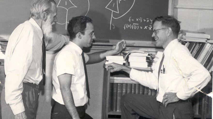
Frank Rosenblatt, a psychologist at the Cornell Aeronautical Laboratory, described the perceptron in 1958. He built on the artificial neuron that Warren McCulloch and Walter Pitts had proposed in 1943: a unit that adds up its inputs and fires when the total passes a threshold. McCulloch and Pitts had to set the weights by hand. Rosenblatt's new idea was a rule that set them from examples. The press was thrilled: in July 1958 the New York Times reported that the Navy expected the machine to walk, talk, see and be conscious of its existence one day.
The Mark I Perceptron
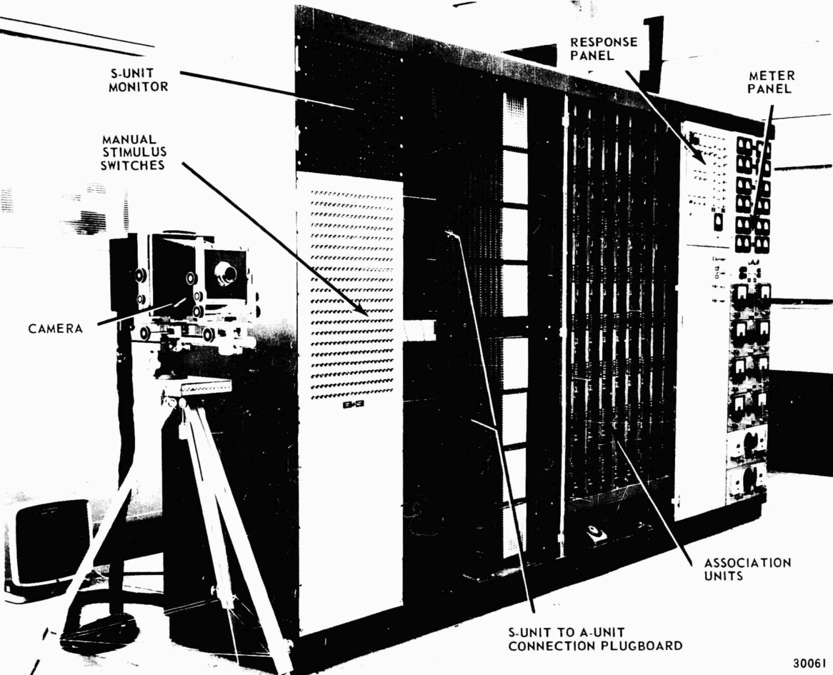
The first perceptron ran as a program on an IBM 704, but Rosenblatt soon had it built as a machine of its own. The Mark I Perceptron, finished around 1960, looked at the world through a camera of 400 light sensors in a 20 by 20 grid, wired at random to a layer of association units. Its weights were potentiometers, turned by small electric motors whenever it made a mistake. It learned to tell simple shapes and letters apart. The machine is now kept at the Smithsonian's National Museum of American History.
One neuron, one straight line
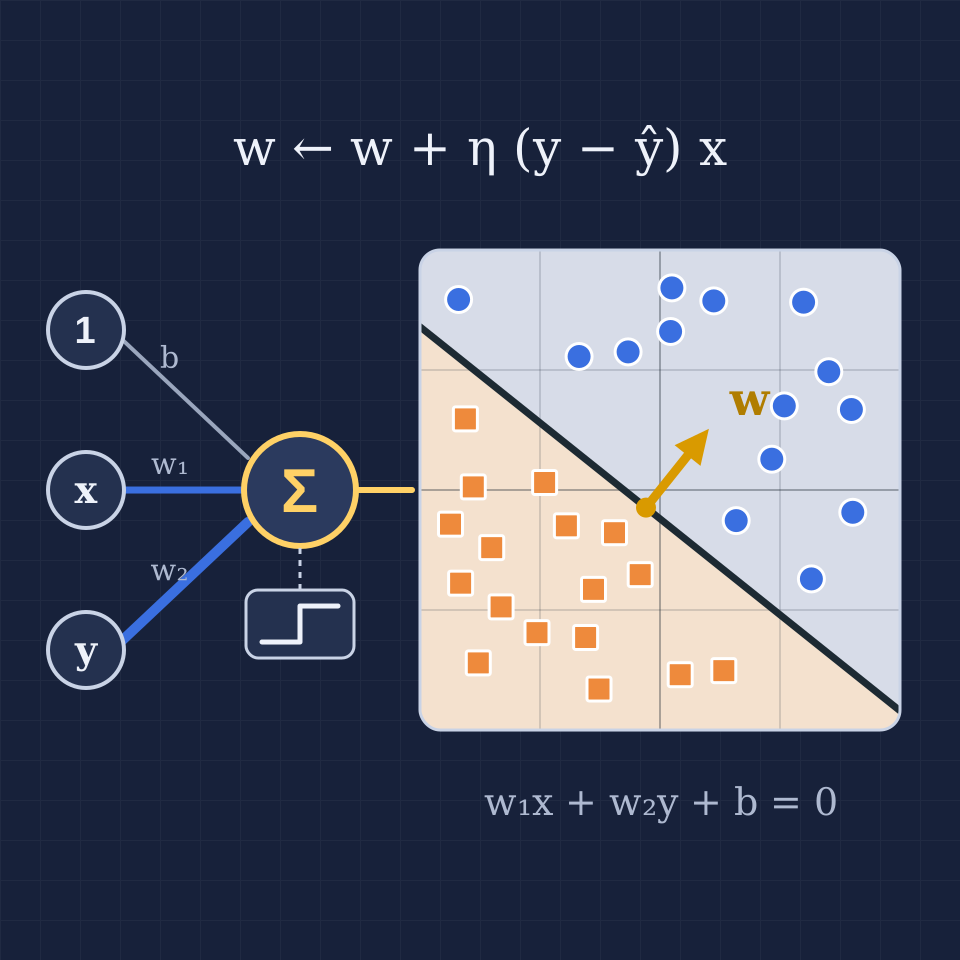
A perceptron with two inputs x and y computes w₁x + w₂y + b and answers +1 if that sum is positive and −1 if it is negative. The sum is zero exactly on the line w₁x + w₂y + b = 0, so the neuron splits the plane into two half-planes, one for each answer. The weight vector (w₁, w₂) is perpendicular to the line and points into the +1 side, and the bias b moves the line away from the origin: without it every boundary would pass through (0, 0). With more inputs the line becomes a plane or a hyperplane, but the idea stays the same. The trick of writing the bias as a weight w₀ on an extra input that is always 1 lets one rule learn all the weights.
The learning rule
Training goes through the examples one by one. For each example x with true class y, the neuron gives its answer ŷ. If ŷ equals y, nothing happens. Otherwise every weight changes by η·(y − ŷ) times its input: w ← w + η·(y − ŷ)·x. For a +1 point answered −1, that adds a multiple of x to w, which raises w·x by a multiple of the squared length of x and pushes the point towards the right side; for a −1 point it does the opposite. The learning rate η sets the size of the step. One pass over all examples is an epoch, and the training ends after a pass without a mistake.
The convergence theorem
If some straight line separates the two classes, the perceptron is guaranteed to find one. Albert Novikoff proved in 1962 that if every input has length at most R and the best line separates the classes with a margin γ, the classic rule makes at most (R/γ)² mistakes, however the examples are ordered. The proof compares two quantities: each mistake makes w line up a bit more with the ideal direction, by at least γ, while the length of w grows only like the square root of the number of mistakes, so the mistakes must run out. The line it finds is just one of many that separate the points, not necessarily the one with the widest gap.
Minsky, Papert and XOR
When no straight line separates the classes, the rule never settles: every line misclassifies some point, and that point drags the line away again. The simplest example is XOR, the function that is true when exactly one of its two inputs is true. In their 1969 book Perceptrons, Marvin Minsky and Seymour Papert proved that single-layer perceptrons cannot compute XOR, nor tell whether a figure is connected, and analysed precisely what they can compute. The book is often blamed for the drop in funding for neural network research in the 1970s, although its authors knew that networks with more layers could do more.
From perceptrons to neural networks
XOR is easy for two layers: one neuron computes OR, another NAND, and a third combines them with AND. The trouble was training the hidden neurons, because a hard threshold gives no hint which way to turn a weight. Replacing the step with a smooth function such as the sigmoid made the error differentiable, and backpropagation, popularised in 1986 by David Rumelhart, Geoffrey Hinton and Ronald Williams, computes how much each weight in every layer contributes to the error. Such multilayer perceptrons, grown deep and wide, are the neural networks of today. For data that one layer cannot separate, Stephen Gallant's pocket algorithm of 1990 at least keeps the best line seen during training.

Explore it
Open the perceptron visualizer to train a perceptron on the logic gates AND, OR and NAND, on random points with a margin of your choice, or on points you click in. Step through the learning rule one sample at a time and read each weight before and after the update, watch the line and the weight vector turn, and follow the mistakes per epoch. Then try XOR and the overlapping clouds, see the perceptron fail to converge, and switch on the pocket algorithm.
Frequently asked questions
Is a perceptron the same as logistic regression?
Both are a single neuron with a straight-line boundary, but they learn differently. The perceptron answers only yes or no and changes its weights only after a mistake. Logistic regression passes the sum through a sigmoid to get a probability and adjusts its weights after every example to make the right answers more likely, so it keeps improving even when all points are already on the right side, and it also settles on data that no line separates.
Why does a perceptron need a bias?
Without a bias, w₁x + w₂y is zero at the origin, so every boundary would pass through (0, 0). The gates AND and OR on the inputs 0 and 1 need a line that misses the origin: for AND, for example, 4x + 2y − 5 = 0 separates (1, 1) from the other three corners. The bias is learned like any other weight, as the weight of an input that is always 1.
Which line does the perceptron find?
Any line that separates the points, depending on the start weights and the order of the examples. It stops as soon as there are no mistakes, so the line often passes close to some points. Support vector machines look for the line with the widest margin instead, and the voted and averaged perceptrons of Yoav Freund and Robert Schapire combine the lines seen during training to generalise better.
What is a multilayer perceptron?
A network of neurons in layers, where each layer's outputs are the next layer's inputs. With a smooth activation function instead of a hard threshold it can be trained by backpropagation and gradient descent. A single hidden layer with enough neurons can approximate any continuous function on a bounded region, and two hidden neurons already solve XOR.
Related tools
Perceptron visualizer
Train Rosenblatt's perceptron in your browser: step through the learning rule one sample at a time, watch the decision boundary and the weight vector move, and see why AND and OR are learned but XOR never is.
Neural network sandbox
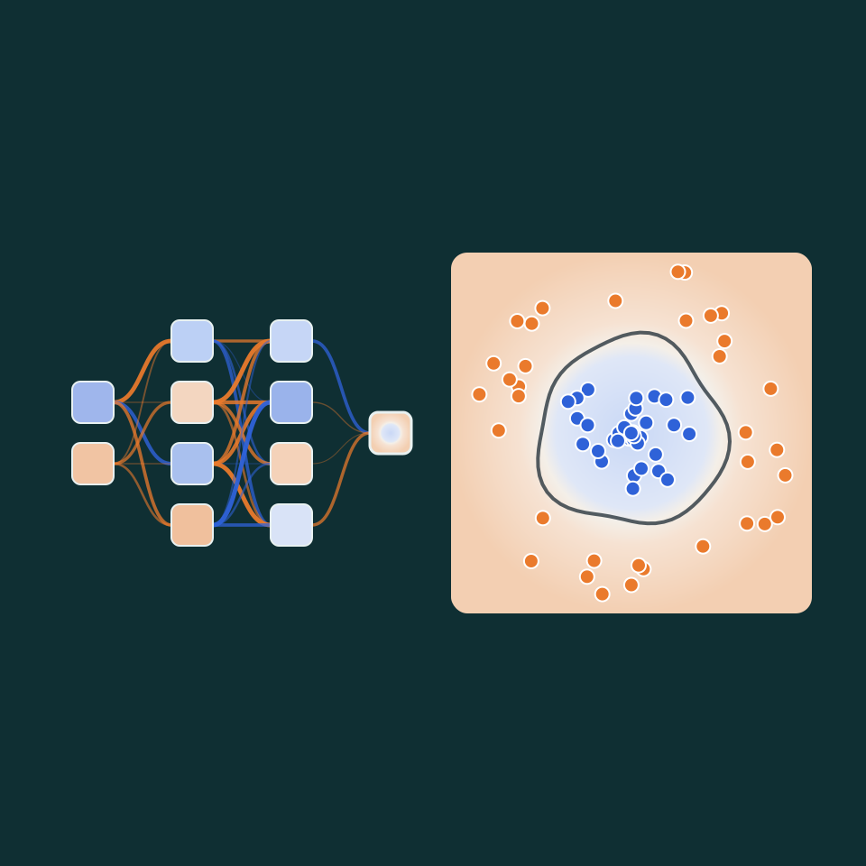
Train a small neural network live and watch it separate two classes of points. Change layers, neurons, activation, learning rate and inputs, and see what every neuron responds to.
Genetic algorithm playground
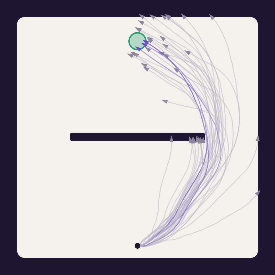
Watch rockets evolve to reach a target round walls. Change population, mutation rate, lifespan and selection, draw your own obstacles, and follow how many arrive in each generation.
Matrix calculator
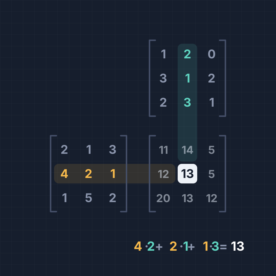
A free online matrix calculator: add, subtract, multiply, transpose and invert matrices up to 6x6, with determinant, rank, powers and exact fractions.
Function plotter
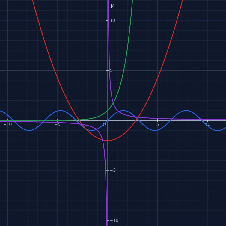
A free online function plotter: draw x², sin x, ln x, 1/x and your own formulas on an interactive grid. Pan, zoom, trace x and y, and save the graph as a PNG.
Ready to try it?
Open PictorX in your browser — no install, no credit card required to start.
Open the perceptron visualizer