
How Simpson's paradox works
Simpson's paradox is a trend that appears in every group of data but reverses when the groups are combined. It is not a trick of the numbers but a warning: a comparison can depend on a third factor that decides who ends up in which group. Here is how it arises, where it has been found and what to do about it.

A trend that flips
In 1995 David Justice had a better batting average than Derek Jeter (.253 against .250), and in 1996 too (.321 against .314). Yet over both years together Jeter was ahead, .310 against .270. The reason: Jeter had most of his at-bats in 1996, his good year, and Justice most of his in 1995, his weaker one. Each player's overall average is pulled towards the year in which he batted most.
The arithmetic behind it
An overall rate is a weighted average of the group rates, and the weights are each option's share of cases in each group. If one option has most of its cases in an easy group and the other in a hard group, the weights can outweigh the differences within the groups. For the kidney stone study: open surgery 0.25 × 93.1% + 0.75 × 73.0% = 78.0%, keyhole surgery 0.77 × 86.7% + 0.23 × 68.8% = 82.6%.
The Berkeley admissions case
In the autumn of 1973, the University of California, Berkeley admitted about 44% of its male graduate applicants and 35% of the female ones. Peter Bickel, Eugene Hammel and William O'Connell looked at the departments separately and published their analysis in Science in 1975. In most departments women were admitted at a similar or higher rate. Women had mostly applied to departments that admitted few applicants of either sex, which pulled their overall rate down. In the six largest departments, men were admitted at 44.5% and women at 30.4%, yet women did better in four of the six.
Which answer is right?
The data alone cannot decide; the way the data came about does. When the grouping factor influences both which option is chosen and the outcome, it is a confounder: doctors chose open surgery more often for large stones, which are harder to treat, so the fair comparison is within stone sizes. When the grouping is itself a consequence of the option, for example a measurement taken after a treatment, splitting by it can hide the effect, and the combined figure is the better guide. The computer scientist Judea Pearl showed how causal diagrams settle the question.
A short history
Karl Pearson and his colleagues noticed the effect in 1899 and George Udny Yule described it in 1903; Edward H. Simpson wrote about it in 1951, and the statistician Colin Blyth named it Simpson's paradox in 1972. It is also called the Yule-Simpson effect, the amalgamation paradox or the reversal paradox. It turns up in medical trials, school results, election analyses and sports statistics alike.
Frequently asked questions
How can I spot Simpson's paradox?
Look at how the cases are spread over the groups. If the options being compared have very different shares of their cases in groups with high and low success rates, the overall comparison can mislead. Split the data by the factor that might drive both, and compare the rates within each group.
Does it only happen with two groups?
No. It can happen with any number of groups, and with continuous data too: a correlation that is positive within every subgroup can be negative across all of them together. Two groups are simply the easiest way to see it.
Was there gender bias at Berkeley?
The 1975 analysis found no bias against women in the departments' decisions; if anything, a small one in their favour. The overall gap came from where women applied: to departments with many applicants and few places. Whether those departments had too few places is a different question that the admission figures cannot answer.
Related tools
Simpson's paradox
Explore Simpson's paradox: see how one option can do better in every group yet worse overall, with real data on kidney stone treatments, Berkeley admissions and batting averages, or your own numbers.

The birthday paradox
In a group of 23 people the chance that two share a birthday is 50.7%, and with 57 people it is 99%. See all 253 pairs, the calendar and the curve, and test thousands of random groups in your browser.

The Monty Hall problem
Pick one of three doors, watch Monty open one with a goat, then stay or switch. Play yourself or let the computer play 1,000 games and see switching win two times out of three.
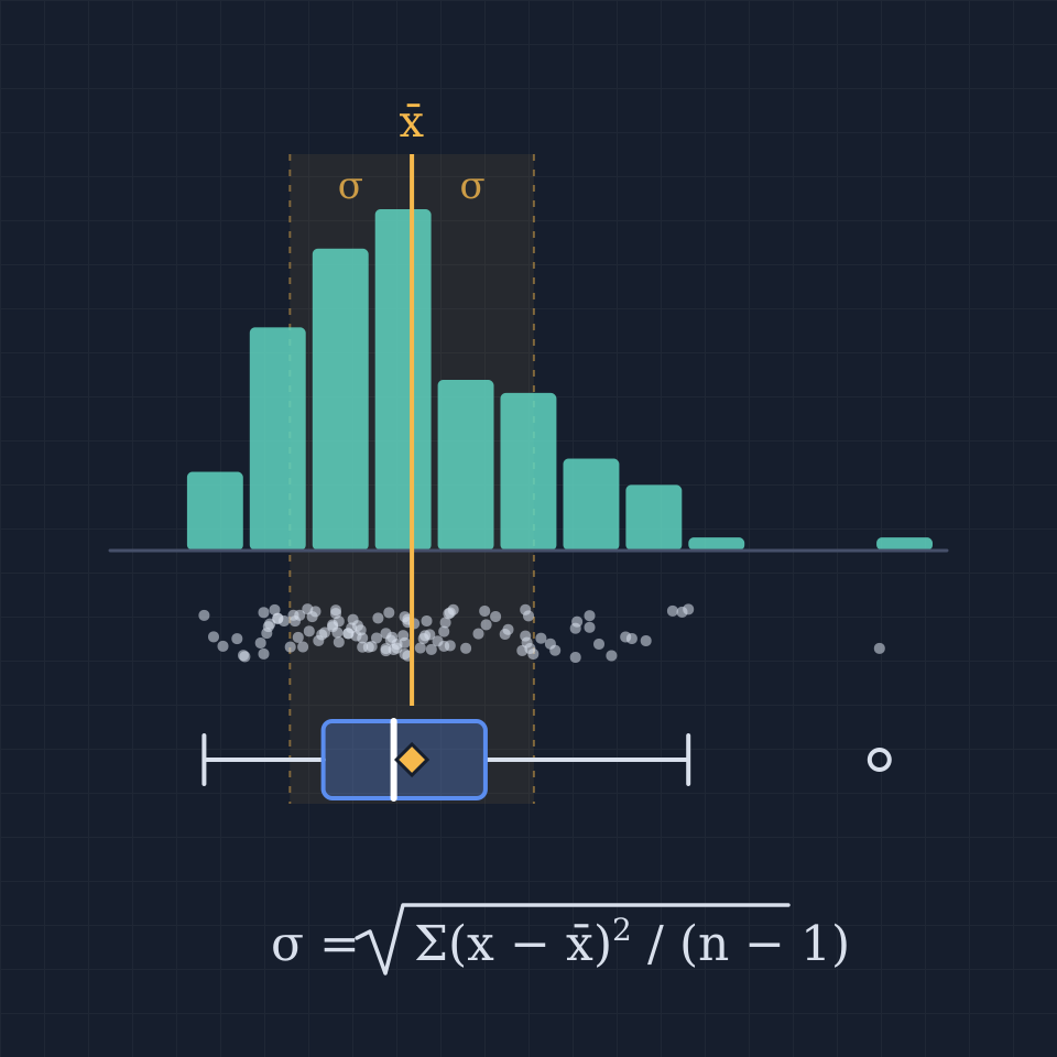
Statistics calculator
A free online statistics calculator: paste numbers and get the mean, median, mode, variance, standard deviation, quartiles and a histogram instantly.
Ready to try it?
Open PictorX in your browser — no install, no credit card required to start.
Open the Simpson's paradox app