
Neural networks explained
The systems that recognise faces, translate text and write answers are built from a surprisingly plain idea: many small units that each add up numbers, bend the result a little, and pass it on. Nobody programs the rules. The network starts with random settings and adjusts them, a tiny step at a time, until its answers match the examples it is shown. This article follows that idea from one neuron to a network that learns a spiral.
One neuron
An artificial neuron takes a few numbers, multiplies each by a weight, adds them up together with a bias, and passes the total through an activation function. Warren McCulloch and Walter Pitts described such a unit in 1943, and in 1958 Frank Rosenblatt built the perceptron, a machine that learned its own weights from examples. With two inputs x and y, the weighted sum is zero along a straight line, so a single neuron splits the plane into two halves: one side is its yes, the other its no, with a soft transition when the activation is smooth.
Activation functions
The activation function is what makes a network more than a sum. The sigmoid squeezes any number into 0 to 1 and tanh into −1 to 1; both are smooth S-shaped curves. ReLU, the rectified linear unit, outputs zero for negative numbers and the number itself otherwise; since about 2010 it has been the usual choice for deep networks because it is cheap and keeps the gradients from fading. Without a bend of this kind, stacking layers would be pointless: a chain of linear functions is still one linear function, and its boundary is still a straight line.
Layers
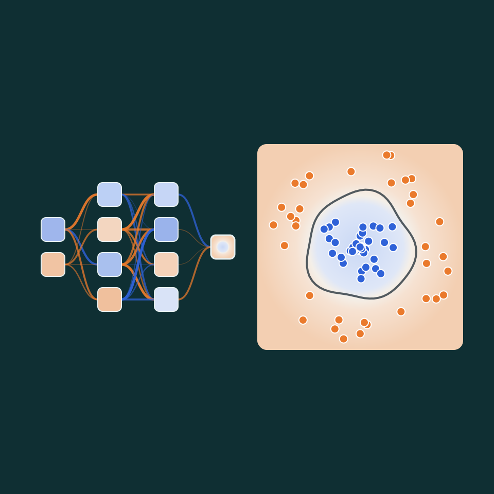
Put several neurons side by side and you have a layer; feed one layer's outputs into the next and you have a network. In the sandbox the first hidden layer cuts the plane along several lines, the next layer combines those half-planes into wedges and islands, and the output neuron weighs it all into one probability. In 1969 Marvin Minsky and Seymour Papert showed that a perceptron without hidden layers cannot learn XOR, which helped bring the field to a standstill for years. Twenty years later George Cybenko and others proved the opposite for networks with one hidden layer: with enough neurons they can approximate any continuous function as closely as you like.
Measuring the error
To learn, a network needs a number that says how wrong it is: the loss. For two classes the usual choice is the cross-entropy. If the network gives a blue point a probability p of being blue, that point costs −log p, which is small when p is near 1 and grows without limit as p approaches 0. The loss is the average cost over the points. A network that guesses one half everywhere has a loss of log 2, about 0.693, close to where the sandbox's chart starts.
Gradient descent and backpropagation
Think of the loss as a landscape over all the weights. Gradient descent finds the downhill direction, the negative gradient, and takes a small step that way, again and again. Computing the gradient for thousands of weights looks expensive, but backpropagation does it in one backward pass: starting from the error at the output, the chain rule hands each layer its share of the blame, layer by layer back to the inputs. The method was described several times, and the 1986 paper by David Rumelhart, Geoffrey Hinton and Ronald Williams made it the standard way to train networks. Using a small random batch of points for each step instead of all of them, stochastic gradient descent, is faster and works just as well.

The learning rate
The step size is called the learning rate, and it is the setting that most often decides whether training works. Too small, and the loss creeps down so slowly that nothing seems to happen. Too large, and each step overshoots the valley it was aiming for: the loss bounces up and down, or in bigger networks explodes until the numbers overflow. With ReLU a large step can also push neurons to where their sum is negative for every point; they then output zero, get no gradient and never recover. Try the spiral with a rate of 3 in the sandbox: with tanh the loss jumps around, with ReLU many neurons go blank and the loss sticks near 0.69. Then try 0.001 to see it crawl.
Overfitting
A network with enough weights can memorise its training points, noise and all, and draw a boundary that twists around every stray point. It then does well on the points it has seen and badly on new ones. That is why part of the data is held back as test data, never used for training. While both losses fall, the network is learning the pattern; when the test loss turns up while the training loss keeps falling, it has started to memorise. Smaller networks, more data, adding noise or simply stopping at the right moment all help.
Explore it
Open the neural network sandbox to train a network of up to four hidden layers of eight neurons on six datasets, including points you click in yourself. Each neuron is drawn as a small map of what it responds to, and each weight as a blue or orange connection, so you can watch the network invent its own features. Try the circle without hidden layers, then add x² and y² as inputs; try the spiral with one layer, then with three; and add noise to a small dataset to make it overfit.
Frequently asked questions
Is this how large AI models work?
The building blocks are the same: weighted sums, activation functions, a loss and gradient descent with backpropagation. Large models have billions of weights instead of a few dozen, layers built for images or text such as convolutions and attention, and they train on huge datasets with better optimisers. The basic loop you see in the sandbox is unchanged.
Why does training start from random weights?
If every weight started equal, every neuron in a layer would compute the same thing and receive the same update, and they would stay identical forever. Small random weights break that symmetry, so each neuron can learn a different feature. Their size matters: the sandbox scales them to the number of inputs, as Xavier Glorot and Yoshua Bengio suggested in 2010.
Why do two runs end with different boundaries?
Each run starts from different random weights and sees the points in a different random order, and the loss landscape has many valleys that are almost equally good. Two networks can classify the training points equally well with differently shaped boundaries, and they may disagree in regions that have no data.
Are more layers always better?
No. Deeper networks can represent more complex shapes with fewer neurons, but they are harder to train and overfit more easily on small datasets. For the problems in the sandbox, one or two hidden layers are usually enough; the spiral is the one that clearly benefits from more.
Related tools
Neural network sandbox
Train a small neural network live and watch it separate two classes of points. Change layers, neurons, activation, learning rate and inputs, and see what every neuron responds to.
Function plotter
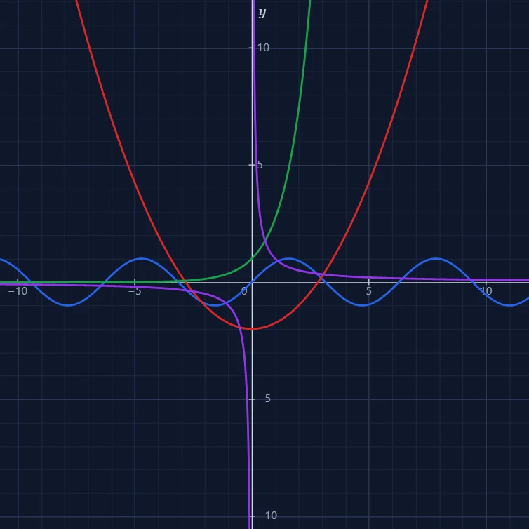
A free online function plotter: draw x², sin x, ln x, 1/x and your own formulas on an interactive grid. Pan, zoom, trace x and y, and save the graph as a PNG.
Matrix calculator
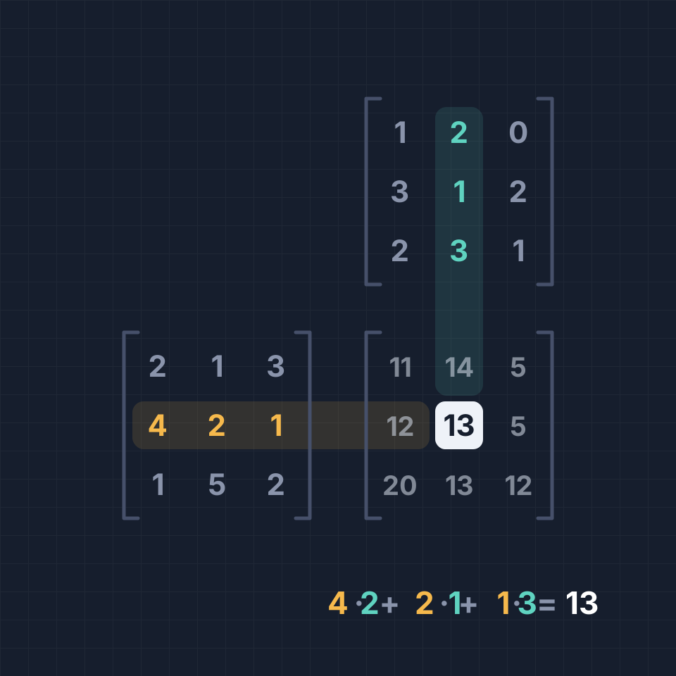
A free online matrix calculator: add, subtract, multiply, transpose and invert matrices up to 6x6, with determinant, rank, powers and exact fractions.
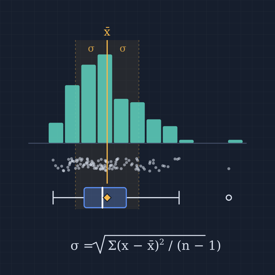
Statistics calculator
A free online statistics calculator: paste numbers and get the mean, median, mode, variance, standard deviation, quartiles and a histogram instantly.
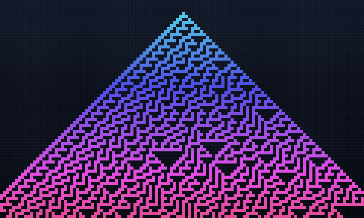
Cellular Automata
Run Conway's Game of Life, Rule 30, Rule 110, Brian's Brain, and Wireworld in your browser. Draw cells, change the rule, and watch simple rules grow complex patterns.
Ready to try it?
Open PictorX in your browser — no install, no credit card required to start.
Open the neural network sandbox